Emoji Journey: Exploring Sentiments with the Power of TPUs 🎉
Notebook: here
Today, I’m excited to share a fun mini project I’ve been working on 🎉. I came across a dataset of tweets with emojis on Kaggle and thought, “Why not try to do something with this?” 🤔. The project started out pretty standard, but as there was a ton of data and my architectures were quite large (I tried transformers again without success - yet again 😅), it quickly became challenging. I attempted to run it on my local GPU, Kaggle, and Google Colab GPUs, but the processing times were just too much (like one hour per epoch 😫). That’s when I decided to venture into something that perhaps you, my dear reader, haven’t tried before: TPUs 💡. And guess what? This made a HUGE difference! 🚀 So, without further ado, let’s dive right in!
Dataset Overview
Alright, let’s take a closer look at the dataset I’m working with in this project 🕵️♀️. The dataset, called emojifydata-en, consists of millions of tweets, each containing emojis 😄. The data is split into four files: train, test, dev, and one file that has everything combined. To get started, I needed to do a bit of preprocessing, as the raw data wasn’t exactly user-friendly. Here are a few example tweets before preprocessing:
<START> O
CeeC O
is O
going O
to O
be O
another O
Tboss O
What O
is O
45 O
million O
Naira 😂
<STOP> O

<START> O
This O
gif O
kills O
me O
Death O
is O
literally O
gushing O
towards O
you O
and O
you O
really O
gon O
do O
a O
whole O
3point O
turn 😩
<STOP> O

<START> O
LOVE O
TEST O
Raw O
Real O
JaDine 💜
<STOP> O
Yes, it’s Twitter, and people don’t always write with perfect grammar 🤷. This adds an extra layer of challenge when creating a language model.
The dataset contains a total of 49 different emoji classes 🌈. Initially, I attempted to create a classifier for all of these classes, but it quickly became apparent that I would need much more data to achieve accurate results. So, I decided to narrow it down to just 5 emojis, ensuring that they represented a diverse range of sentiments. The emojis I chose are: 🤦, 🤣, 🙏, 😩 and 🤔. By selecting these distinct emojis, I hoped to give the classifier a better chance at accurately predicting the sentiment behind each tweet.
Preprocessing
In the dataset, each tweet is separated with one word per line, and each word ends with an “O” unless there’s an emoji, in which case the line ends with the emoji 📝. Each tweet is also delimited by START and STOP tokens that have an “O” attached. To make the data more manageable, I first reconstructed the tweets from this format into complete sentences. During this process, I noticed that some tweets contained more than one emoji, so I only kept the content up until the first emoji that appeared 🚧. If a tweet started with an emoji, it resulted in an empty sentence, which I discarded. Next, I performed some basic preprocessing, such as lowercasing and removing symbols, and filtered the tweets to keep only those containing my chosen emojis.
As I mentioned earlier, Twitter users tend to have quite creative spelling 🎨. I wanted to tackle this issue by using machine learning to correct spelling errors. I found a project called Neuspell that aims to do just that. Unfortunately, I encountered difficulties running the project and, when I finally got it to work, it was too slow for my needs (taking about a second per tweet, and I have hundreds of thousands) ⏳.
Model
Initially, this post was going to compare Transformers and RNNs, but I struggled to train a Transformer successfully 🤖. Despite trying finetuning, no finetuning, and battling OOM errors in both RAM and GPU, I only achieved a slow-improving model that seemed like it would never finish. So, I abandoned the Transformer and decided to explore an architecture with GRUs and Attention layers instead.
  inputs = Input(shape=(32))
  embedding = Embedding(input_dim=4096, output_dim=1024, input_length=max_length)(inputs)

  out_layer = embedding
  for i in range(2):
    gru = GRU(1024, activation='relu', return_sequences=True)(out_layer)
    batch_norm = BatchNormalization()(gru)
    dropout = Dropout(0.5)(batch_norm)
    attention = Attention()([dropout, dropout])
    out_layer = Concatenate(axis=-1)([dropout, attention])

  gru = GRU(512, activation='relu')(out_layer)
  batch_norm = BatchNormalization()(gru)
  dropout = Dropout(0.5)(batch_norm)

  outputs = Dense(5, activation='softmax')(dropout)
This architecture isn’t overly complex. The layer sizes and overall structure are quite experimental 🧪. Although I read that using a ’tanh’ activation for GRU layers was recommended, I found that ‘relu’ worked better in my case. Adding Attention layers proved to be a significant improvement 📈.
Here is the summary:
__________________________________________________________________________________________________
 Layer (type)                   Output Shape         Param #     Connected to
==================================================================================================
 input_1 (InputLayer)           [(None, 32)]         0           []

 embedding (Embedding)          (None, 32, 1024)     4194304     ['input_1[0][0]']

 gru (GRU)                      (None, 32, 1024)     6297600     ['embedding[0][0]']

 batch_normalization (BatchNorm  (None, 32, 1024)    4096        ['gru[0][0]']
 alization)

 dropout (Dropout)              (None, 32, 1024)     0           ['batch_normalization[0][0]']

 attention (Attention)          (None, 32, 1024)     0           ['dropout[0][0]',
                                                                  'dropout[0][0]']

 concatenate (Concatenate)      (None, 32, 2048)     0           ['dropout[0][0]',
                                                                  'attention[0][0]']

 gru_1 (GRU)                    (None, 32, 1024)     9443328     ['concatenate[0][0]']

 batch_normalization_1 (BatchNo  (None, 32, 1024)    4096        ['gru_1[0][0]']
 rmalization)

 dropout_1 (Dropout)            (None, 32, 1024)     0           ['batch_normalization_1[0][0]']

 attention_1 (Attention)        (None, 32, 1024)     0           ['dropout_1[0][0]',
                                                                  'dropout_1[0][0]']

 concatenate_1 (Concatenate)    (None, 32, 2048)     0           ['dropout_1[0][0]',
                                                                  'attention_1[0][0]']

 gru_2 (GRU)                    (None, 512)          3935232     ['concatenate_1[0][0]']

 batch_normalization_2 (BatchNo  (None, 512)         2048        ['gru_2[0][0]']
 rmalization)

 dropout_2 (Dropout)            (None, 512)          0           ['batch_normalization_2[0][0]']

 dense (Dense)                  (None, 5)            2565        ['dropout_2[0][0]']

==================================================================================================
Total params: 23,883,269
Trainable params: 23,878,149
Non-trainable params: 5,120
Running Environments
I’d like to mention that for this project, I experimented with three different environments: my local PC (good CPU, 48GB RAM, 6GB GPU), Google Colab, and Kaggle Notebooks 🖥️.
Each option has its pros and cons. While my PC isn’t as powerful as the other two instances, I can run my model overnight without worrying about being disconnected. Google Colab and Kaggle offer less RAM (around 15GB) but more powerful GPUs. However, I can’t run a process for too long on them. The real game-changer comes in the form of TPUs.
So, what are TPUs? TPUs (Tensor Processing Units) are specialized hardware accelerators designed by Google specifically for machine learning 💡. They are optimized to perform matrix operations and are especially effective for training and running large neural networks. TPUs can provide significant speedups compared to traditional CPUs and GPUs, making them an invaluable resource for accelerating machine learning applications.
While I can’t afford to buy a TPU since I’m not a millionaire yet 💸, both Colab and Kaggle allow you to use theirs. So what’s the difference? My model on a GPU takes one hour per epoch, but on a TPU… it takes 70 seconds ⚡.
Setting up TPUs
First of all, how do you gain access to a TPU? 🤔
Kaggle makes it easy by providing it as an option right from the start. Simply change the Accelerator to TPU VM v3-8 in the Notebook options. There’s a high demand for these instances, so you might have to wait a bit – on average, I waited 15 minutes. If you’re #20 or less in the queue, just be patient; it’ll be worth your while. Another great feature is that the instance comes with 330GB RAM (yes, you read that correctly) 🎉.
For Google Colab, you’ll need to request access here. I got it on the same day. The advantage here is that there’s less demand, and it’s unlikely that you’ll have to wait for the TPU. However, you won’t have 330GB of RAM, just the usual 15GB-ish.
Once you have an environment with a TPU, setting up the code is a breeze. Just execute this once:
tpu = tf.distribute.cluster_resolver.TPUClusterResolver.connect()
tpu_strategy = tf.distribute.experimental.TPUStrategy(tpu)
And then wrap your model compilation within this statement:
with tpu_strategy.scope():
    model = Sequential()
    ...
    ...
    model.compile(...)
And that’s it 🚀.
Now, with a TPU comes great power: you can use a large batch_size like 1024 and parallel batches with the steps_per_execution parameter in the compile method:
model.compile(optimizer=optimizer,
			  loss=loss_fn,
			  metrics=metrics,
			  steps_per_execution=32)
And we can draw more power. Kaggle documentation on TPUs say:
Because TPUs are very fast, many models ported to TPU end up with a data bottleneck.
The TPU is sitting idle, waiting for data for the most part of each training epoch.
Even with all our previous efforts, the TPU can still be idle (!). Kaggle TPUs read from GCS (Google Cloud Storage) and their solution to this bottleneck is to feed the TPU with several GCS files in parallel. I haven’t tried this approach, so I’m not sure if it’s easy or not. However, it’s certainly a potential method to explore if you want to further optimize your TPU utilization.
Results
I trained the model for 30 epochs, and thanks to the TPU, each epoch took only 70 seconds 🚀. The validation accuracy I achieved was 0.6 without Attention layers and 0.7 with Attention. Another thing I tried was measuring the accuracy of the top 2 results, since two emojis could be acceptable for a given text 🤔. This approach yielded an accuracy of around 0.85, but I ultimately decided to stick with the traditional accuracy measure.
Here are some results predicted by the model from the validation set:
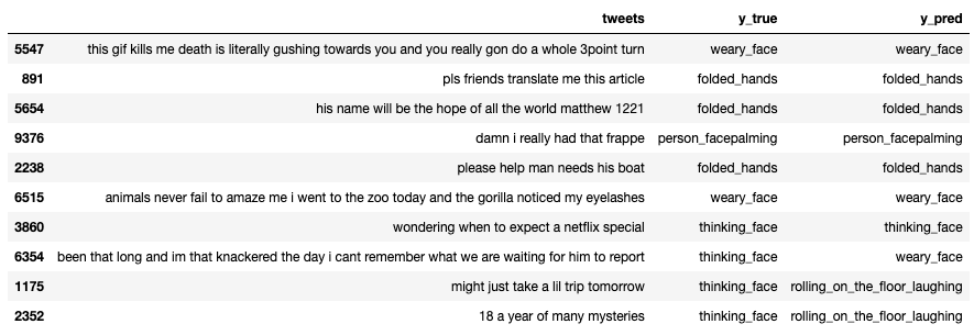
And here is a csv extract of the results, if you want to explore
Conclusion
In conclusion, TPUs have been a game changer for this project and I can confidently say that I’ll be using them in future projects as well 🌟. The incredible speedup they provide allows me to train models much faster, making experimentation and iteration far more feasible.
The accuracy of the emoji classification model, while not perfect, is still acceptable given the nature of the task and the inherent challenges of dealing with social media text. However, it is important to remember that the primary goal of this post was to showcase the power of TPUs, rather than solely focusing on the emoji classification problem.
Thanks for reading!
Notebook: here