Painting with pixels: Variational Autoencoders applied to art
Introduction
This time around, I felt the urge to explore the world of VAEs (Variational Autoencoders). These autoencoders can be used for generating new data, but we’ll get into that in a bit. I wanted to avoid the all-too-common MNIST example, so I opted for a more adventurous route: generating ⭐art!⭐ This experiment could either be a smashing success or an entertaining disaster. So, let’s dive into this artistic adventure with VAEs…
 ⭐Art!⭐
What is a Variational Autoencoder?
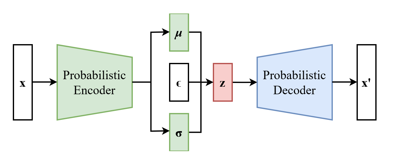 VAE architecture (from Wikipedia)
Autoencoders
Imagine you’re trying to send a message to a friend, but you need to use as few words as possible. You’d want to find a way to compress your message into a shorter form that still conveys the essential information. Then your friend would like to elaborate on your summarized information to reconstructthe original message. Autoencoders work in a similar way. They are unsupervised neural networks that learn to compress and then reconstruct data, much like you would with your message.
An autoencoder has two main parts: the encoder and the decoder. Picture the encoder as a master of summarization, while the decoder is an expert at elaborating on the summary.
Encoder
The encoder is likes to summarize. It takes the input data and distills it into a brief summary (called latent space representation). This summary captures the essence of the data, but in a much more compact form. The goal of the encoder is to represent the input data in the most concise and efficient way possible, without losing too much information.
Decoder
On the other hand, the decoder is like a storyteller who takes the summary (latent space representation) and reconstructs the full original data from it. The decoder aims to recreate the original data as accurately as possible, using only the information provided in the summary.
Autoencoders learn to perform these tasks by minimizing the difference between the input data and the reconstructed data. By doing so, they become effective at tasks like data compression, denoising, feature extraction, and representation learning.
Today, we’re exploring representation learning. Our aim is to find a useful way to represent our images, so we can create new ones that share similar features with the original images.
Adding the variation and latent space
While traditional autoencoders can learn to compress and reconstruct data, they might not be the best choice for generating new, high-quality samples. This is where Variational Autoencoders (VAEs) come into play. VAEs add a probabilistic twist to the autoencoder framework, making them more suitable for generating diverse and realistic samples.
In a regular autoencoder, the latent space is usually a small Dense layer. But this fixed layer has a drawback: once trained, it always gives the same output for the same input, making its behavior deterministic.
In a VAE, we handle the latent space as if it were a game of chance. This means that every time we use an input, the output has a random element, so it’s not always the same. For the same input, we can get different outputs that still are in the trained data space. Our plan is to train the VAE with images and let its random nature create a variety of interesting results.
Instead of using a Dense layer, we incorporate two layers, μ and σ, which represent the parameters of a normal distribution. This way, we compress our images into a Gaussian-shaped space. When evaluating the model, we place a step between the encoder and decoder that involves sampling a random variable from the normal distribution using μ and σ. This sampled variable is then used to modify the input to the decoder.
This looks easy until you have to train it… How do you do backpropagation with non deterministic layers? (spoiler: you don’t)
Reparametrization trick
Remember that we’re representing our input in a compressed form (latent space) and in a stochastic manner (due to the μ and σ layers). However, we can’t perform backpropagation like this. The reparameterization trick is a clever technique used to enable gradient-based optimization in models like VAEs that involve stochastic sampling from a distribution. It helps us backpropagate through the random sampling process in the latent space by transforming it into a deterministic operation.
In a VAE, we have two components in the latent space: μ and σ, which represent the mean and standard deviation of a normal distribution, so far so good. To sample a latent variable, we would typically generate a random value from this distribution. However, this random sampling is not differentiable, and we cannot backpropagate the gradients through it.
The reparameterization trick comes to the rescue by separating the random sampling process from the model parameters. Instead of directly sampling from the normal distribution, we sample a random variable epsilon from a standard normal distribution (with a mean of 0 and standard deviation of 1). We then scale this random variable by the learned standard deviation (σ) and add the learned mean (μ). Mathematically, it looks like this:
z = mu + sigma * epsilon
Now, the sampling process becomes a deterministic operation: μ and σ are model parameters like any other. When the time comes to generate a random sample, we use epsilon (that is not a model parameter). This transformation allows gradients to flow through the model during backpropagation, enabling the optimization of VAEs using gradient-based methods.
Loss function
Another important component of our VAE is the loss function. How do we measure correctness of our process?
In a Variational Autoencoder, the loss function has two main parts, which set it apart from the loss function in a regular autoencoder. The two parts of the VAE loss function are the reconstruction loss and the KL-divergence loss.
Reconstruction loss: The reconstruction loss checks how well the VAE can rebuild the input data. This part of the loss makes sure that the output created is as close to the original input as possible. Depending on the input data, we can use metrics like Mean Squared Error or Binary Cross-Entropy for the reconstruction loss. This reconstruction loss is what traditional autoencoders use. You have a message that you compress and want to get the original message again, so your measure of correctness should be how close is your message to the original one.
KL-divergence loss: This is the special sauce of the VAE loss function and… kinda hard to explain (maybe for another post). Basically, it measures how different the learned distribution in the latent space (controlled by μ and σ) is from a standard normal distribution (with a mean of 0 and standard deviation of 1). The KL-divergence loss acts like a gentle nudge, guiding the learned distribution closer to the standard distribution. This helps create a smooth and continuous structure in the latent space, which is great for generating new samples.
On the other hand, a regular autoencoder only cares about the reconstruction loss, aiming to minimize the difference between the input data and the output. By adding the KL-divergence loss, a VAE focuses not just on the quality of reconstruction but also on building a well-structured latent space. This makes VAEs perfect for tasks like generating new data and smoothly transitioning between samples.
This is the formula for the KL-divergence loss. It could seem daunting but it is a matter of just coding it into the model.
$$ \frac{1}{2} \left[ \left(\sum_{i=1}^{z}\mu_{i}^{2} + \sum_{i=1}^{z}\sigma_{i}^{2} \right) - \sum_{i=1}^{z} \left(log(\sigma_{i}^{2}) + 1 \right) \right] $$
VAE implementation
Getting the implementation done took a bit of effort. I initially aimed to work with CVAEs (VAEs with convolutional layers). Despite giving it my best shot, I couldn’t quite get it to work as expected. So, I decided to stick with standard VAEs for now. Perhaps in the future, I’ll explore more powerful models like GANs or diffusion models to tackle this challenge.
The implementation is simple, just the Encoder, Decoder, loss function and putting it all together in a VAE class.
Encoder
The Encoder is relatively straightforward, consisting of three Dense layers that progressively decrease in size and two Dense layers that represent μ and σ.
class Encoder(Model):
    def __init__(self, latent_dim):
        super(Encoder, self).__init__()
        self.dense1 = layers.Dense(512, activation='relu')
        self.dense2 = layers.Dense(256, activation='relu')
        self.dense3 = layers.Dense(128, activation='relu')
        self.dense_mean = layers.Dense(latent_dim)
        self.dense_log_var = layers.Dense(latent_dim)

    def call(self, inputs):
        x = self.dense1(inputs)
        x = self.dense2(x)
        x = self.dense3(x)
        mean = self.dense_mean(x)
        log_var = self.dense_log_var(x)
        return mean, log_var
Decoder
The Decoder follows the reverse path compared to the Encoder, going from smaller to larger layers. Keep in mind that the input to the Decoder is the random variable z.
z = mu + sigma * epsilon
class Decoder(Model):
    def __init__(self, original_dim):
        super(Decoder, self).__init__()
        self.dense1 = layers.Dense(128, activation='relu')
        self.dense2 = layers.Dense(256, activation='relu')
        self.dense3 = layers.Dense(512, activation='relu')
        self.dense_output = layers.Dense(original_dim, activation='sigmoid')

    def call(self, z):
        x = self.dense1(z)
        x = self.dense2(x)
        x = self.dense3(x)
        output = self.dense_output(x)
        return output
VAE
Putting it all together looks like this:
class VAE(Model):
    def __init__(self, encoder, decoder, latent_dim):
        super(VAE, self).__init__()
        self.encoder = encoder
        self.decoder = decoder
        self.latent_dim = latent_dim

    def call(self, inputs):
        mean, log_var = self.encoder(inputs)
        epsilon = tf.random.normal(shape=(tf.shape(inputs)[0], self.latent_dim))
        z = mean + tf.exp(log_var * 0.5) * epsilon
        reconstructed = self.decoder(z)
        return reconstructed, mean, log_var
Loss function
A quick recap, the loss function for a VAE has two main components: reconstruction loss and KL divergence.
Reconstruction loss: This is a standard binary crossentropy loss calculated for each pixel (or element) in the input image, which ensures the accurate reconstruction of the input data. It is multiplied by the image shape.
KL divergence: The KL divergence is calculated using a previously mentioned formula and acts as a regularization term.
def vae_loss(inputs, reconstructed, mean, log_var):
    reconstruction_loss = tf.reduce_mean(tf.keras.losses.binary_crossentropy(inputs, reconstructed)) * 28 * 28
    kl_loss = -0.5 * tf.reduce_sum(1 + log_var - tf.square(mean) - tf.exp(log_var), axis=-1)
    return tf.reduce_mean(reconstruction_loss + kl_loss)
Art Attack
Alright, let’s dive in! We’ll be using a dataset of art masterpieces to train our Variational Autoencoder. By doing so, we hope to create a model that can generate visually appealing and diverse artistic images. Fingers crossed!
Goal and expectations
First, let’s set some expectations. Our goal is to use a non-convolutional VAE to generate complex images. A convolutional VAE would be more appropiate but I couldn’t make it work on my side. Also with a limited dataset of around 10k diverse images, we shouldn’t expect fully-formed, novel paintings. However, if the model can capture the general form and colors of a painting, I’ll consider it a win.
Data and examples
I’ll be utilizing the wikiart dataset courtesy of Huggingface. This dataset features a variety of artists, genres, and styles. To help the model, I’ll filter the dataset to use only landscapes, as mixing different categories like portraits and landscapes would require more data for the model to differentiate between them. Also, I made some tests with the classic MNIST to see that everything is ok before feeding it the art images.
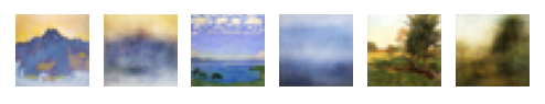
Lets see some examples:
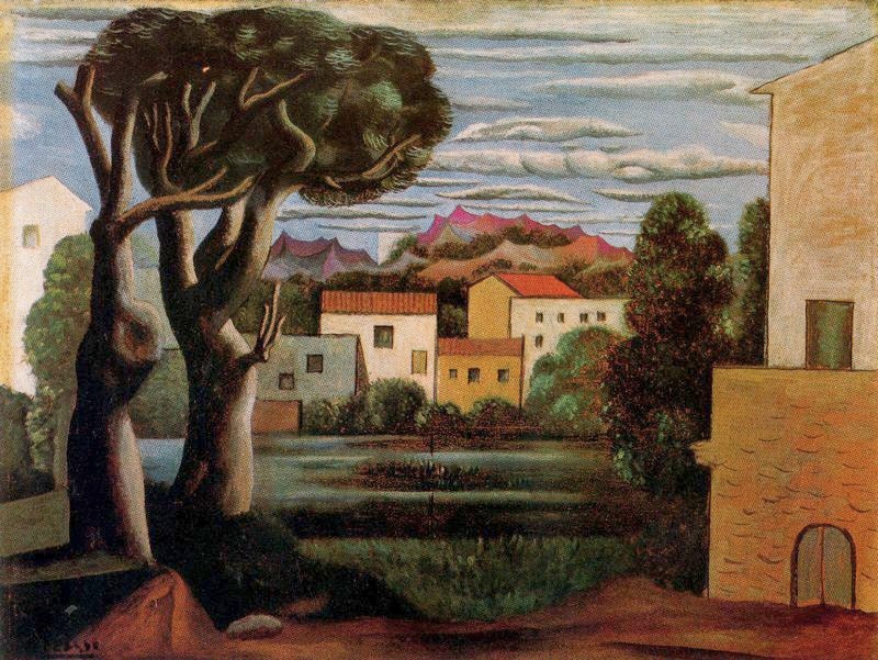
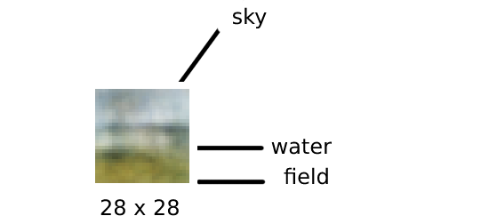
 Example 1
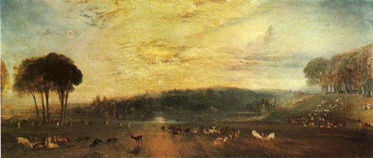
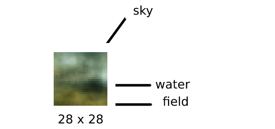
 Example 2
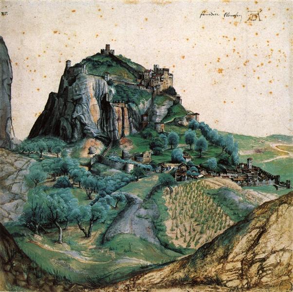
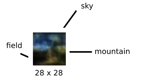
 Example 3
Training
First I used MNIST to check eveything went correctly and it did
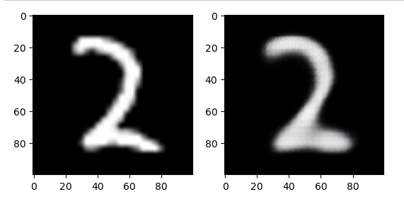
The original image vs the reconstruction
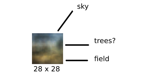
MNIST uses 28 * 28 pixel greyscale images, so I resized my art images to 28 * 28 and transformed them into grayscale. The results were somewhat satisfactory, but a bit blurry. The main issue was that it was difficult to see anything in such small images without colors. To address this, I reintroduced the RGB channels, which effectively tripled the input size, making everything slower. However, I was able to train 200 epochs in a couple of hours locally.
Here is the training step used
# Instantiate and compile the VAE
latent_dim = 64
encoder = Encoder(latent_dim)
decoder = Decoder(3*28*28)
vae = VAE(encoder, decoder, latent_dim)
optimizer = tf.keras.optimizers.Adam(lr=0.001)

# Train the VAE
epochs = 200
batch_size = 100

for epoch in range(epochs):
    print(f"Epoch {epoch+1}/{epochs}")
    for i in range(0, len(train_ds), batch_size):
        x_batch = np.array(train_ds[i:i+batch_size]['pixel_values']).reshape((-1, 3*28*28))
        with tf.GradientTape() as tape:
            reconstructed, mean, log_var = vae(x_batch)
            loss = vae_loss(x_batch, reconstructed, mean, log_var)
        gradients = tape.gradient(loss, vae.trainable_variables)
        optimizer.apply_gradients(zip(gradients, vae.trainable_variables))
    print(loss)
Remember that latent_dim is the size of our μ and σ layers. I used latent_dim=2 for MNIST and that was ok, but my problem needed more dimensions so I decided for latent_dim=64.
Generating art
Lets look now at the results.
First the reconstruction results, I feed the VAE with existing images and I should get the reconstructed image.
Hey not bad! It is a very blurry but I can see the shape and color of each image, this is a win. ⭐Blurry Art!⭐
Now I feed the decoder only with random normal values that represent the z variable. I use the weights for μ and σ and added a generated epsilon.
Generated image 1
Generated image 2
Generated image 3
Generated image 4
Conclusion
Alright, I consider this a win, even if we didn’t create a new masterpiece. The blurriness of the images is likely due to insufficient training and the fact that the architecture is not convolutional. In the future, I’d like to experiment with a GAN or a diffusion model, if possible. There are also other exciting projects to explore, such as generating 3D objects. Imagine creating a valid 3D object that can be fed into Blender and then printed with a 3D printer!
Additionally, there are other types of VAEs like beta-VAE and VQ-VAE that I might try for other topics, such as text generation. Thank you all for sticking with me through this lengthy post, and I’ll see you next time!
Here is the link to the Notebook